As hardware gets faster and more capable, software keeps getting slower. It is remarkable how inefficiently typical apps use the capabilities of modern processors! Often this means an app is doing only one thing at a time when it could do multiple things simultaneously, even on a single thread.
This article explores a technique for doing more than one thing at a time by vectorizing the code. We will use a puzzle from Advent of Code 2024 to provide a realistic scenario to experiment on.
Vectorizing means using processor instructions that work on many pieces of data (a vector of values) at the same time. These instructions are called SIMD instructions and they come with terms and conditions attached, which means they are rarely automatically used by the compiler. We need to write our code differently to make use of SIMD instructions.
To illustrate, what we are talking about is a faster way to perform calculations such as (in pseudocode):
X[0] = A[0] + B[0]
X[1] = A[1] + B[1]
X[2] = A[2] + B[2]
X[3] = A[3] + B[3]
Vectorized code can issue a single instruction to achieve all of this at once (in pseudocode):
X[0..4] = A[0..4] + B[0..4]The main practical impact is that when we are looping over a data set, we can speed up the loop by processing multiple loop iterations at the same time.
Note: for complete code samples that you can compile and benchmark, refer to GitHub – sandersaares/vectorized-rust. Snippets below may omit less relevant content and detailed comments in the interest of readability.
This is not multithreading
It is worth emphasizing that everything in this article is happening in the context of a single thread running on a single logical processor (a single CPU core) – nothing described here is related to multithreading, which is a separate but unrelated technique for doing more than one thing at a time.
For optimal performance, you would typically want to combine vectorized code with multithreading, doing many things at the same time on many threads. This combined technique is out of scope of this article.
This is not async
It is also worth emphasizing that nothing is this article is related to async/await. Asynchronous code is code that an executor automatically switches in and out of execution based on the readiness of futures but asyncronous logic only ever executes one task at a time per thread, with the other tasks waiting for their turn or for an external event. It is an independent technique for orchestrating work and is not relevant in scope of this article.
This is not hyper-threading
Yet another mechanism for doing multiple things at the same time is hyper-threading, which allows two threads to execute at the same time on the same processor. In the interest of clarity, this is also an independent mechanism completely unrelated to this article.
What are we vectorizing here?
The scenario under exploration is puzzle 13 from Advent of Code 2024. This is a simple algebra exercise that can be solved without any loops but for the purposes of this article we are going to pretend we do not understand algebra and will solve the puzzle by brute force, directly evaluating every potential solution until we find what we are looking for.
The puzzle boils down to a system of two equations with unknown variables A and B:
Xa * A + Xb * B = X
Ya * A + Yb * B = Y
We must find the solution with the minimal value for A (which implies there can be multiple solutions), with the two unknown variables being nonnegative integers and the constants being positive integers. There may be systems of equations presented with no solution.
Example inputs:
Xa = 94
Xb = 22
X = 11613264
Ya = 34
Yb = 67
Y = 4202904
The iterative algorithm to solve this is quite simple:
- Identify the maximum possible value for
Ato establish the upper bound for the search.- The maximum value is identified by looking for the threshold where
Bwould have to become negative (which is not allowed).
- The maximum value is identified by looking for the threshold where
- For each candidate
Ain0..=max_a, verify the following:- Do both equations yield an integer value for
B(i.e. divides without remainder)? - Do both equations yield the same value for
B?
- Do both equations yield an integer value for
- The first (lowest) candidate value for A that satisfies both criteria is our solution.
The expected output in our example scenario consists of the values for A and B. The original puzzle further elaborates it with some additional calculations derived from these two values but we can ignore that part of the puzzle. The solution can be represented as the following Rust type:
The solution for example inputs is:
A = 123536
B = 40
Implemented in Rust code, this naive algorithm becomes:
This algorithm works correctly but will require evaluating many iterations of the loop, possibly millions or billions, depending on the constants given in the puzzle. We are deliberately not going to avoid executing these iterations but we will try to make them as fast as we can by vectorizing the code.
Automatic vectorization
The compiler has built-in heuristics to identify vectorizable parts of code. If it sees a loop that applies the same calculation to each iteration, without any dependencies between iterations, then it may decide to transform that code to vectorized code. No changes needed by the author – a free performance optimization!
Alas, this is only rarely applicable and often still requires a helping hand by the author to nudge the compiler in the right direction. There are many preconditions to automatic vectorization, which make it inapplicable in the scenario we are exploring.

Most importantly, our loop iterations are not independent! If we return Some(_) from our loop evaluation function, we break the loop! This is an implicit return statement in find_map(), creating a dependency between iterations – if one iteration returns, the next will not execute! This immediately disqualifies the code from automatic vectorization.
Furthermore, our loop iterations are not executing the same calculation for each element – we have if-statements that terminate the calculation early if certain conditions are met, by returning None and skipping the rest of the evaluation function body. Again, this disqualifies the code from automatic vectorization.
As these examples illustrate, automatic vectorization is narrowly constrained to apply only in specific scenarios. Sometimes it is possible to make small adjustments to the logic to enable automatic vectorization but this is still a limited approach. We are not going to rely on automatic vectorization for our app – instead, we will be quite explicit about our expectations for the compiler.
Manual vectorization
The limitations of automatic vectorization are not due to shortcomings of the compiler but rather a fundamental aspect of vectorized logic – it is a technique for applying the same calculations to many values at the same time. The same calculations. This eliminates the possibility of continue, break or return statements being executed for some of the loop iterations because these would change the calculations performed in that loop iteration!
We must therefore find a shape for our algorithm that processes each loop iteration with the exact same logic while still giving us the final results we are looking for.
First, we need to restructure our loop into working on chunks of our input values instead of individual loop iterations – we process CHUNK_SIZE iterations at the same time, where CHUNK_SIZE is the vector instruction parallelism factor supported by our target processor’s instruction set. For now, we will set CHUNK_SIZE=4, which is a reasonable default for processing 64-bit values on modern processors that support the 256-bit AVX2 instruction set.
We need to add a LaneCount<CHUNK_SIZE>: SupportedLaneCount constraint to prove to the compiler that our chunk size is within the range the compiler supports for vector operations.
What if our loop iteration count is not evenly divisible by CHUNK_SIZE? The standard technique here is to fall back to the naive non-vectorized algorithm for the last partial chunk. Only full chunks are processed in vectorized mode. Yes, this means our app must contain two versions of the loop processing code. This will also prove useful for other reasons further below.
There are different techniques for transforming our if/continue/return based logic to vectorized form but a very useful approach is to separate processing of each chunk into two stages:
- A series of identical vector calculations applied to the chunk of
CHUNK_SIZEloop iterations. - A post-processing stage that performs the “
if-statement logic” for each chunk ofCHUNK_SIZEloop iterations.
A key insight we can use for finding a suitable transformation is that most loop iterations will not yield a valid solution – for the example inputs given earlier, only the 123537th iteration yielded a solution! In other words, if we can come up with a way to say “none of the iterations in this chunk are a valid solution” without any if-statements or other branching logic, we have a useful vectorized form already! Then when the evaluation of a chunk yields the opposite result (“at least one iteration in this chunk is a valid solution”) we can simply fall back to the slower naive algorithm to find the solution in that chunk. After all, 99.99% of the work is already done by that point and the speed of the last 0.01% does not matter.
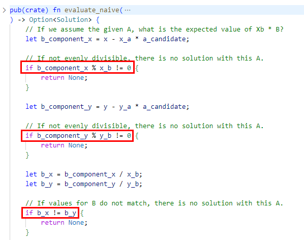
We can accomplish this by transforming all our if-statements into branchless boolean algebra, evaluating each loop iteration as the following pseudocode:
is_evenly_divisible_x= does theBcomponent of theXformula divide evenly to yield an integer value forB?is_evenly_divisible_y= does theBcomponent of theYformula divide evenly to yield an integer value forB?are_expressions_equal= do both equations give the same value forB?return is_evenly_divisible_x && is_evenly_divisible_y && are_expressions_equal
This is branchless logic because we are simply executing the same boolean algebra for each loop iteration. Later in the post-processing stage we can check the return values to answer the question “did any iteration in this chunk return true” – if yes, we can identify which of them returned true and use the naive algorithm to determine the B component of the solution.
Let’s implement this. The first thing we need is a way to represent our data in a form suitable for vectorized calculations. This is the std::simd::Simd type, which is conceptually similar to an array that includes an extra set of behaviors required to enable the compiler to use vector instructions. It can be used as a numeric type for the purpose of mathematical operations.
Mathematical SIMD operations take vectors of values as inputs, even if all you are doing is multiplying many values with the same factor. In most cases, both operands to a SIMD operation must be vectors. In our case, this specifically refers to our constants, which we must convert to vector form before using. Simd::splat() will give us a vector filled with the same value, repeated.
Note that the size of the vectors we operate on (our chunk size) must be provided as a generic parameter to the Simd type, with the full signature being Simd<u64, CHUNK_SIZE>. This is inferred from (omitted) usage in the snippet above.
Converting our evaluate_naive() to a vectorized evaluate_chunk() gives us the following function for evaluating one chunk of candidate values for A:
This also uses the Mask type, which is a sibling of the Simd type for boolean algebra – think of it as a vector of arbitrarily-sized booleans. The i64 in the generic type constraints is there just to match the size of the values in the vectors we are operating on – it is not actually a numeric type.
The result of this evaluation can then be post-processed to yield the actual solution, with the full form of solve() being:
What is the speedup?
We have now converted the code into a vectorized form, making it substantially more complex. The price has been paid; now, what is the benefit?
Let’s execute some Criterion benchmarks to measure the effect with “cargo bench”:
Note: the use of black_box() stops the compiler from being too clever and making optimizations that depend on the specific input values we give it. Always wrap benchmark inputs/outputs in this to ensure you are benchmarking the general case and not seeing an effect specific to optimizations from the input values you are using.
The results are straightforward:
| Algorithm | Time taken (μs) | Time taken (vs naive) |
|---|---|---|
| Naive | 180.37 | |
| Vectorized | 383.76 | +113% |
Wait, what? The vectorized code is much slower!? Yes, that’s right – we made our code more complex and significantly slower, gaining nothing at all and, in fact, making things worse.
This finding serves to highlight two important factors:
- We must always measure the impact of our changes; we cannot simply assume that following some cargo cult advice from the internet makes things better!
- Optimization is a journey – things will often get worse before they get better. Be prepared for the long road if you want to get to the destination.
Our journey is not yet complete – clearly, we still have some distance to go. The next step is to understand what exactly is happening when our vectorized algorithm is executed – where is the time spent? Learning this will give us the hints we need to make further changes on the path to great success.
Getting what we paid for
A very useful tool to understand what the hardware is doing is Intel VTune. If you are not on an Intel system, fear not – the most important functionality is also supported on non-Intel processors. Guidance on use of this tool is out of scope of this article. We can build the following simple binary to analyze what is happening when our algorithm is executed:
For high quality output in VTune, we need to add the following into cargo.toml:
[profile.release]
debug = "full"
Let’s run this binary under the Hotspots analysis in VTune. The calculation above will run for around 5-10 minutes on a modern computer, giving us plenty of data to analyze. It should also be fine to stop the analysis sooner (or make the X/Y constants smaller) if you want to rush things along.
If we click through to the evaluate_chunk() function in the analysis and enable the assembly view, we observe something that immediately raises a red flag:
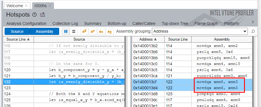
The xmm registers are being used! This is a red flag because xmm registers are 128-bit registers. Our CHUNK_SIZE is 4 and we are using 64-bit integers, which means we have 4*64=256 bits of data. Efficiently operating on this requires the use of 256-bit registers. Indeed, you see two instructions highlighted above, first moving 128 bits of data and then moving a different 128 bits of data – that is our single chunk, split in two for no good reason!
The processor the author is using is capable of 256-bit operations but for some reason the app is not using the full capabilities of the hardware. We should be seeing it use ymm registers instead. You can easily identify this from the names of the registers you see used:
| Register name | Register size (bits) |
|---|---|
xmm* | 128 |
ymm* | 256 |
zmm* | 512 |
The reason for this is simple. Consider, how does the compiler know what instructions are legal to use? Different processors have different capabilities! By default, the Rust compiler is conservative and only uses up to 128-bit instructions because some modern processors might lack support for wider instructions.
There are multiple techniques that can be used to overcome this limitation. The most popular options are:
- Compile multiple versions of the relevant functions and select the optimal version after checking the processor capabilities at runtime.
- Hardcode the processor capabilities at compile time and simply do not support processors that lack those capabilities.
The former is more flexible but out of scope of this article. For our purposes, we will go with the latter option. To enable 256-bit operation support at compile time, define the following environment variable before building the project:
RUSTFLAGS="-C target-feature=+avx,+avx2"Note that if the resulting binary is executed on a processor that lacks 256-bit instructions then it will crash.
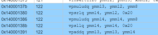
That’s better – we now see the ymm registers used, proving that 256-bit instructions are in use. If we scroll around in the assembly view, we still see xmm used here and there but the presence of ymm registers in many of the instructions proves that they are enabled, which is enough for now. What changes in our benchmarks?
| Algorithm | Time taken (μs) | Time taken (vs naive) |
|---|---|---|
| Naive | 180.37 | |
| Vectorized (128-bit) | 383.76 | +113% |
| Vectorized (256-bit) | 360.46 | +99% |
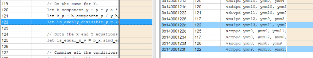
Not much, really – the vectorized code is still very slow! Let’s continue digging into what the processor is doing. Reading further in the assembly code of evaluate_chunk() shows some instructions that do not follow the general pattern of using ymm registers. In fact, some instructions do not even use xmm registers! This is our next hint that something is still fishy.

We have hit another snag here. We are using the u64 integer data type for our values but it is an unfortunate truth that integer division is very complicated/expensive to implement in hardware. There are no SIMD instructions for integer division at all! To divide integers, they must be taken out of the vectors, divided individually with the div instruction, and the result inserted back into the vectors. All of that is slow.
There is no generally applicable way to get rid of the division when working with integers. However, with some analysis of our problem space, we can obtain a key insight to make further progress: all algorithm steps for our valid solutions consist of integer operations and are within the “safe f64” range (i.e. our values do not require more than 53 bits of data to represent). This means for valid solutions, all values – including inputs, outputs and intermediate values – are representable without precision loss as 64-bit floating point values.
Floating point values do support fast vectorized division via SIMD instructions! While there are precision problems when dealing with non-integer (or very large) values stored in floating point representation, we are not affected by these as long as all our input and output values are integers that fit within 53 bits of data, and as long as we only perform basic mathematical operations on them (add, subtract, multiply, divide). For iterations that are not valid solutions, non-integer values may be present and suffer from precision issues but we do not need to care about those iterations, at least for the purposes of solving our target Advent of Code puzzle.
Therefore, let’s convert our algorithm to use f64 for all its internal logic, only using u64 at the public API boundary. This gives us fast vectorized division and still yields the correct results:
Finally, we see some good news on the benchmarks:
| Algorithm | Time taken (μs) | Time taken (vs naive) |
|---|---|---|
| Naive | 180.37 | |
| Vectorized (128-bit, u64) | 383.76 | +113% |
| Vectorized (256-bit, u64) | 360.46 | +99% |
| Vectorized (256-bit, f64) | 69.04 | -62% |
Great success! We now have an algorithm that is faster by a good margin and can be confident knowing that our investment into optimization has paid off.
Still, additional opportunities for performance gain may remain! If you can find ways to squeeze even more performance out of the app, please leave a comment below.
Unstable all the things
We got the performance we were looking for but unfortunately, this technique is not applicable in many scenarios due to non-technical reasons. This is because the Rust language and standard library hide many useful features behind feature flags marked as unstable, which forces us to use the nightly toolchain to enable the features. This is often impossible in enterprise environments, where the nightly toolchain cannot be used for various policy reasons.
This severely limits the value of the affected Rust platform features, especially as Rust features often stay in unstable form for years and years with little movement toward stabilization. Unfortunately, the Simd type is one of these unstable features, requiring a nightly toolchain that allows the programmer to enable the portable_simd feature flag required by this type.
There is a tendency in Rust toward a proliferation of “forever unstable” features which is a major obstacle holding back the Rust ecosystem from achieving a solid foothold in the enterprise domain. There does not seem to be a general solution to this problem today given Rust’s community-driven nature. There is no company acting as the driving force behind Rust and the people paid to improve Rust for the platform’s benefit remain few – if you depend on such features in an enterprise context where unstable tooling cannot be used, you will need to invest the money and engineering time to drive such features toward stability yourself.
There exist 3rd party crates that try to offer similar functionality for stable Rust toolchains, so all is not lost. However, use of these crates is out of scope of this article.
Additional reading
Single instruction, multiple data – Wikipedia
pulp – crates.io: Rust Package Registry
wide – crates.io: Rust Package Registry
safe_arch – crates.io: Rust Package Registry
